Time series (astropy_timeseries)
Introduction
Many different areas of astrophysics have to deal with 1D time series data,
either sampling a continuous variable at fixed times or counting some events
binned into time windows. The astropy_timeseries package therefore provides
classes to represent and manipulate time series
The time series classes presented below are QTable sub-classes that have
special columns to represent times using the Time class. Therefore, much of
the functionality described in Data Tables (astropy.table) applies here.
Getting Started
In this section, we take a quick look at how to read in a time series, access the data, and carry out some basic analysis. For more details about creating and using time series, see the full documentation in Using timeseries.
The simplest time series class is TimeSeries - it represents a time series as
a collection of values at specific points in time. If you are interested in
representing time series as measurements in discrete time bins, you will likely
be interested in the BinnedTimeSeries sub-class which we show in
Using timeseries).
To start off, we retrieve a FITS file containing a Kepler light curve for a source:
>>> from astropy.utils.data import get_pkg_data_filename
>>> filename = get_pkg_data_filename('timeseries/kplr010666592-2009131110544_slc.fits')
We can then use the TimeSeries class to read in this file:
>>> from astropy_timeseries import TimeSeries
>>> ts = TimeSeries.read(filename, format='kepler.fits')
Time series are specialized kinds of Table objects:
>>> ts
<TimeSeries length=14280>
    time             timecorr   ...   pos_corr1      pos_corr2
                        d       ...     pixels         pixels
   object            float32    ...    float32        float32
----------------------- ------------- ... -------------- --------------
2009-05-02T00:41:40.338  6.630610e-04 ...  1.5822421e-03 -1.4463664e-03
2009-05-02T00:42:39.187  6.630857e-04 ...  1.5743829e-03 -1.4540013e-03
2009-05-02T00:43:38.045  6.631103e-04 ...  1.5665225e-03 -1.4616371e-03
              ...           ... ...            ...            ...
2009-05-11T18:05:14.479  1.014664e-03 ...  3.5986886e-03  3.1407392e-03
2009-05-11T18:06:13.328  1.014689e-03 ...  3.5967610e-03  3.1329831e-03
2009-05-11T18:07:12.186  1.014713e-03 ...  3.5948332e-03  3.1252259e-03
In the same way as for Table, the various columns and rows can be accessed and
sliced using index notation:
>>> ts['sap_flux']
<Quantity [1027045.06, 1027184.44, 1027076.25, ..., 1025451.56, 1025468.5 ,
           1025930.9 ] electron / s>

>>> ts['time', 'sap_flux']
<TimeSeries length=14280>
          time             sap_flux
                         electron / s
         object            float32
----------------------- --------------
2009-05-02T00:41:40.338  1.0270451e+06
2009-05-02T00:42:39.187  1.0271844e+06
2009-05-02T00:43:38.045  1.0270762e+06
                    ...            ...
2009-05-11T18:05:14.479  1.0254516e+06
2009-05-11T18:06:13.328  1.0254685e+06
2009-05-11T18:07:12.186  1.0259309e+06

>>> ts[0:4]
<TimeSeries length=4>
          time             timecorr   ...   pos_corr1      pos_corr2
                              d       ...     pixels         pixels
         object            float32    ...    float32        float32
----------------------- ------------- ... -------------- --------------
2009-05-02T00:41:40.338  6.630610e-04 ...  1.5822421e-03 -1.4463664e-03
2009-05-02T00:42:39.187  6.630857e-04 ...  1.5743829e-03 -1.4540013e-03
2009-05-02T00:43:38.045  6.631103e-04 ...  1.5665225e-03 -1.4616371e-03
2009-05-02T00:44:36.894  6.631350e-04 ...  1.5586632e-03 -1.4692718e-03
As seen in the example above, TimeSeries objects have a time
column, which is always the first column. This column can also be accessed using
the .time attribute:
>>> ts.time
<Time object: scale='tcb' format='isot' value=['2009-05-02T00:41:40.338' '2009-05-02T00:42:39.187'
 '2009-05-02T00:43:38.045' ... '2009-05-11T18:05:14.479'
 '2009-05-11T18:06:13.328' '2009-05-11T18:07:12.186']>
and is always a Time object (see Times and Dates), which
therefore supports the ability to convert to different time scales and formats:
>>> ts.time.mjd
array([54953.0289391 , 54953.02962023, 54953.03030145, ...,
       54962.7536398 , 54962.75432093, 54962.75500215])

>>> ts.time.unix
array([1.24122482e+09, 1.24122488e+09, 1.24122494e+09, ...,
       1.24206503e+09, 1.24206509e+09, 1.24206515e+09])
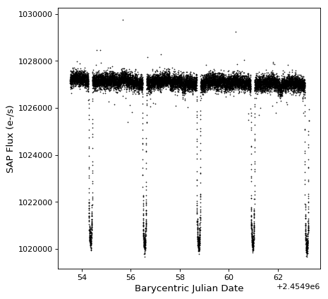
Let’s use what we’ve seen so far to make a plot
import matplotlib.pyplot as plt
plt.plot(ts.time.jd, ts['sap_flux'], 'k.', markersize=1)
plt.xlabel('Barycentric Julian Date')
plt.ylabel('SAP Flux (e-/s)')

It looks like there are a few transits! Let’s use
BoxLeastSquares to estimate the period, using a box with
a duration of 0.2 days:
>>> import numpy as np
>>> from astropy import units as u
>>> from astropy.stats import BoxLeastSquares
>>> keep = ~np.isnan(ts['sap_flux'])
>>> periodogram = BoxLeastSquares(ts.time.jd[keep] * u.day,
...                               ts['sap_flux'][keep]).autopower(0.2 * u.day)
>>> period = periodogram.period[np.argmax(periodogram.power)]
>>> period
<Quantity 2.20551724 d>
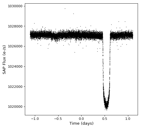
We can now fold the time series using the period we’ve found above using the
fold() method:
>>> ts_folded = ts.fold(period=period, midpoint_epoch='2009-05-02T07:41:40')
Let’s take a look at the folded time series:
plt.plot(ts_folded.time.jd, ts_folded['sap_flux'], 'k.', markersize=1)
plt.xlabel('Time (days)')
plt.ylabel('SAP Flux (e-/s)')
Using the Astrostatistics Tools (astropy.stats) module, we can normalize the flux by sigma-clipping the data to determine the baseline flux:
>>> from astropy.stats import sigma_clipped_stats
>>> mean, median, stddev = sigma_clipped_stats(ts_folded['sap_flux'])
>>> ts_folded['sap_flux_norm'] = ts_folded['sap_flux'] / median
and we can downsample the time series by binning the points into bins of equal
time - this returns a BinnedTimeSeries:
>>> from astropy_timeseries import simple_downsample
>>> ts_binned = simple_downsample(ts_folded, 0.03 * u.day)
>>> ts_binned
<BinnedTimeSeries length=74>
  time_bin_start      time_bin_size    ...   pos_corr2    sap_flux_norm
                            s          ...
       object            float64       ...    float32        float32
------------------- ------------------ ... -------------- -------------
-1.1024637743446593             2592.0 ...  -0.0007693809     1.0000684
-1.0724637743446592 2591.9999999999905 ...  0.00038625093     1.0000265
-1.0424637743446594 2592.0000000000095 ...  0.00031359284     1.0000247
-1.0124637743446594             2592.0 ...  0.00017846933     1.0000288
-0.9824637743446593             2592.0 ...  -6.542908e-05    0.99999636
-0.9524637743446593             2592.0 ... -2.9231509e-05     1.0000253
-0.9224637743446593             2592.0 ...   9.763808e-05     1.0000322
-0.8924637743446593             2592.0 ...  0.00012931376     1.0000411
-0.8624637743446593 2592.0000000000023 ...  -0.0011244675     1.0000389
                ...                ... ...            ...           ...
 0.8175362256553407 2591.9999999999977 ...  -0.0006246633     1.0000035
 0.8475362256553407 2592.0000000000014 ...  -0.0006362205     1.0000261
 0.8775362256553407  2592.000000000019 ... -0.00089895696     1.0000074
  0.907536225655341 2591.9999999999814 ...  -0.0008507269     1.0000023
 0.9375362256553407   2592.00000000002 ...  -0.0009239185     1.0000565
 0.9675362256553409  2591.999999999981 ... -0.00020750743     1.0000125
 0.9975362256553407 2592.0000000000095 ... -0.00055085105     1.0000396
 1.0275362256553409 2591.9999999999905 ...  -0.0005766208     1.0000231
 1.0575362256553407             2592.0 ... -0.00023155387     1.0000265
 1.0875362256553407             2592.0 ...  1.5008554e-06    0.99995804
Let’s take a look at the final result:
plt.plot(ts_folded.time.jd, ts_folded['sap_flux_norm'], 'k.', markersize=1)
plt.plot(ts_binned.time_bin_start.jd, ts_binned['sap_flux_norm'], 'r-', drawstyle='steps-post')
plt.xlabel('Time (days)')
plt.ylabel('Normalized flux')
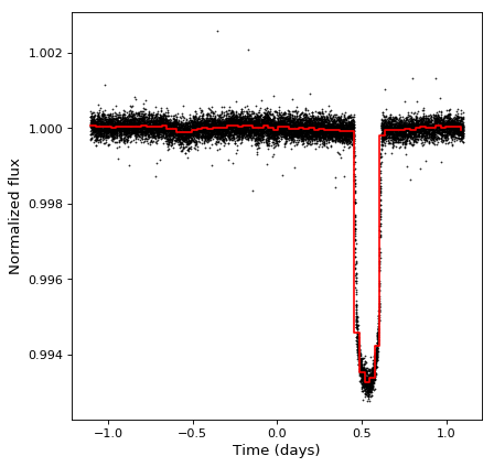
It looks like there might be a hint of a secondary transit!
To learn more about the capabilities in the astropy_timeseries module, you can
find links to the full documentation in the next section.
Using timeseries
The details of using astropy_timeseries are provided in the following sections:
Initializing and reading in time series
Accessing data and manipulating time series
Reference/API
astropy_timeseries Package
This subpackage contains classes and functions for work with time series data sets.
Functions
simple_downsample(time_series, time_bin_size) |
Downsample a time series by binning values into bins with a fixed size, |
test(**kwargs) |
Run the tests for the package. |
Classes
BaseTimeSeries([data, masked, names, dtype, …]) |
|
BinnedTimeSeries([data, time_bin_start, …]) |
|
TimeSeries([data, time, time_delta, n_samples]) |